
Towards Cost Transparency: Estimating Transaction Costs for Smart Beta Strategies
Introduction
It is well known that it is important to account for transaction costs in the evaluation of smart beta investment strategies. Indeed, these strategies have raised concerns due to their higher turnover and higher exposure to illiquid stocks compared to cap-weighted market indices1. Clearly, higher transaction costs are a likely "side-effect" of smart beta strategies and the reasonable question is whether these side-effects outweigh the benefits. However, surprisingly little is known about the magnitude of these costs. In this article, we draw on Scientific Beta research to provide estimates of transaction costs for Scientific Beta indices.
Smart beta strategies are commonly analysed on the basis of backtested performance. Typical backtest results do not consider real life transaction costs. Index providers sometimes state that adjusting the performance of their indices for transaction costs is not something that they can do easily and they prefer to leave it to market participants to figure out what the shortfall would be. This is curious. We would not imagine that pharmaceutical companies advertise drugs while saying that it is up to patients to figure out what the side-effects are.
Thus, in the area of smart beta, there is a need to improve transparency of transaction costs. While studies and reports about transaction costs do exist, providers often rely on arbitrary assumptions on transaction cost levels (such as fixed costs irrespective of the time period or the type of stock that is traded). In both cases, there is not even an attempt to provide explicit estimates of costs.
Research results introducing particular smart beta strategies rarely contain estimates of transaction costs. It is common to present the outperformance of smart beta strategies over cap-weighted indices without subtracting the transaction costs due to portfolio rebalancing.
Studies that take into account implementation issues have either used proprietary data for estimating transaction costs2, rendering the results non-replicable by investors, or analysed generic strategies that are expensive to implement because they do not use turnover controls and are invested in illiquid universes of stocks3. Furthermore, most research focused on strategies invested in the United States, meaning that it is even less clear what the effects of implementation costs on performance for strategies invested in other geographical regions are.
Thus, it has become standard practice for smart beta providers to either estimate these costs using non-replicable methodologies relying on proprietary data, or to leave entirely up to users the burden of measuring these costs.
We think that the current state of affairs is not satisfactory. Therefore, we exploit recent advances in the academic literature on microstructure to provide estimates of costs that draw on easily available public data and are not computationally intensive. Our estimates are thus transparent and easily replicable by investors or other third parties. We argue that such methods to estimate transaction costs should be used widely to increase the transparency of implementation costs in the industry. We use cost estimates to measure the net outperformance of investable smart beta indices in different regional markets with different levels of liquidity. Finally, we analyse the determinants of variation in transaction costs, such as geographic regions, factors or time trends. We show that geographic regions are the main driver of cost variation. This implies that investors who want to diversify away a rising transaction costs shock may benefit from diversification across regions.
Estimating Transaction Costs: Using Transparent and Replicable Methods
Trading costs lower the price for sellers of securities and increase the price for buyers, relative to a market where trading would be frictionless. Total trading costs can be decomposed into three components: the spread, the price impact, and commissions.
The spread reflects the cost of a round trip trade (buy and sell). The basic cost definition is the percent quoted spread which reflects the percentage cost of buying at the ask quote and selling at the bid quote. The percent effective spread is a more useful measure since it accounts for price impact. This measure is based on the (absolute) deviation of the transaction price from the frictionless price (the bid/ask midpoint). The deviation is then multiplied by two so as to reflect round trip costs. Large orders will create a price impact which is captured by the effective spread. For example, a large buy order may lead to an increase of the price beyond the ask quote displayed when the trade was initiated. Such price impact is captured by the effective spread. Huang and Stoll (1996) provide a method for decomposing the effective spread into price impact and the so-called realised spread with the latter reflecting the cost of order processing and inventory risk. Spread measures in principle can be derived from observing the intraday trades and quotes and calculating volume weighted averages across all trades occurring for a security within a trading day.
We define the effective spread of stock j at time t as follows:
Effective Spreadjt = Realised Spreadjt + Price Impactjt
Another source of transaction costs is commissions that brokers may charge for routing orders to market places. However, such commissions are not visible in quotes and transactions and may be difficult to account for since commission schedules may vary widely depending on contractual arrangements and the bargaining power of investors.4
Our main focus in this study is to capture the effective spread component because it can be reliably estimated from market data.
Even when it comes to the spread component, studies of transaction costs of smart beta are rare because accurate estimation of transaction costs in principle requires intraday high frequency data. We need to observe trades and quotes within the trading day to come up with cost measures. However, such data is difficult to access and requires immense computing power given the large number of high frequency trades and quotes.
Recent research has shown that there are effective ways of estimating transaction costs from lower frequency (daily) data. The advantage of such approaches is that results can be generated for longer periods and different markets, with relative computational ease and limited data needs.
There is a fairly broad set of competing methods that allow estimates of effective spreads to be extracted from daily data. Most methods are based on a simple intuition: TC introduce frictions in the price path (e.g. autocorrelation, increase in intraday range). We can thus back out the effective spread by observing the price path.
While there is evidence that the different measures are good proxies of transaction costs5, recent advances in the empirical microstructure literature have introduced new ways of estimating transaction costs from low frequency data which dominate the earlier ones in terms of ability to proxy for high frequency estimates of transaction costs.
In particular, Corwin and Schultz (2012) develop a method which measures bid ask spreads based on the daily price range (high and low prices within the trading day) and Chung and Zhang (2014) use the bid/ask spread quoted at the close of the day as an estimate. Corwin and Schultz (2012) and Chung and Zhang (2014) provide evidence that their new spread measure provides more reliable estimates of effective bid/ask spreads compared to other low frequency methods.
We employ the Chung and Zhang (2014) method for the period for which we have data (from December 1993 to December 2017) and the Corwin and Schultz (2012) methodology to extend our analysis further in time (from December 1977).
Net-of-Cost Performance of Smart Beta Indices
Now we may apply the methodologies that we described previously to smart beta strategies. We first provide a brief description of the indices that are the object of our analysis. Then, we analyse the turnover of these strategies, showing that it is higher than those observed for cap-weighted indices, but still contained to reasonable levels that preserve investability. Finally, we show the estimates of the transaction costs and compare the net and the gross outperformance of our strategies relative to a cap-weighted benchmark.
Description of Strategies and Data
Our objective is to study the transaction costs of investable strategies. Therefore, we analyse commercially available index strategies reflecting seven types of smart beta strategies, namely a mid cap index (MidCap), a value index (Value), a high momentum index (HighMom), a low volatility index (LowVol), a high profitability index (HighProf), a low investment index (LowInv) and a multi-factor index strategy (MBMS6EW). A detailed description of the characteristics of these indices can be found in Amenc and Goltz (2018) and on the www.scientificbeta.com website. In exhibit 1, we report the names of all the Scientific Beta strategies used in our analysis.
In the first part of our study, we use data for the period December 2002 to December 2017 as this is the period for which the data are available from Scientific Beta6 for all the indices and all the regions. We consider indices constructed with stocks of seven regions: United States, United Kingdom, developed Europe ex-UK, Japan, developed Asia ex-Japan, emerging markets and finally a global region. Then, we also study the net outperformance for a longer period but we limit our analysis to the United States as it is the only universe for which we have data for the period from 1977 to 2017.
Exhibit 1: Strategy Names
Region |
Label |
Name |
United States
|
HFI MBMS6EW 4S |
High-Factor-Intensity Diversified Multi-Beta Multi-Strategy 6-Factor 4-Strategy EW |
United States
|
HFI LowVol 4S |
High-Factor-Intensity Low-Volatility Diversified Multi-Strategy (4-Strategy) |
| United States | HFI MidCap 4S | High-Factor-Intensity Mid-Cap Diversified Multi-Strategy (4-Strategy) |
| United States | HFI Value 4S | High-Factor-Intensity Value Diversified Multi-Strategy (4-Strategy) |
| United States | HFI HighMom 4S | High-Factor-Intensity High-Momentum Diversified Multi-Strategy (4-Strategy) |
| United States | HFI HighProf 4S | High-Factor-Intensity High-Profitability Diversified Multi-Strategy (4-Strategy) |
| United States | HFI LowInv 4S | High-Factor-Intensity Low-Investment Diversified Multi-Strategy (4-Strategy) |
| United Kingdom | HFI MBMS6EW 4S |
High-Factor-Intensity Diversified Multi-Beta Multi-Strategy 6-Factor 4-Strategy EW |
| United Kingdom | HFI LowVol 4S |
High-Factor-Intensity Low-Volatility Diversified Multi-Strategy (4-Strategy) |
| United Kingdom | HFI MidCap 4S | High-Factor-Intensity Mid-Cap Diversified Multi-Strategy (4-Strategy) |
| United Kingdom | HFI Value 4S | High-Factor-Intensity Value Diversified Multi-Strategy (4-Strategy) |
| United Kingdom | HFI HighMom 4S | High-Factor-Intensity High-Momentum Diversified Multi-Strategy (4-Strategy) |
| United Kingdom | HFI HighProf 4S | High-Factor-Intensity High-Profitability Diversified Multi-Strategy (4-Strategy) |
| United Kingdom | HFI LowInv 4S | High-Factor-Intensity Low-Investment Diversified Multi-Strategy (4-Strategy) |
| Dev. Europe ex UK | HFI MBMS6EW 4S |
High-Factor-Intensity Diversified Multi-Beta Multi-Strategy 6-Factor 4-Strategy EW |
| Dev. Europe ex UK | HFI LowVol 4S |
High-Factor-Intensity Low-Volatility Diversified Multi-Strategy (4-Strategy) |
| Dev. Europe ex UK | HFI MidCap 4S | High-Factor-Intensity Mid-Cap Diversified Multi-Strategy (4-Strategy) |
| Dev. Europe ex UK | HFI Value 4S | High-Factor-Intensity Value Diversified Multi-Strategy (4-Strategy) |
| Dev. Europe ex UK | HFI HighMom 4S | High-Factor-Intensity High-Momentum Diversified Multi-Strategy (4-Strategy) |
| Dev. Europe ex UK | HFI HighProf 4S | High-Factor-Intensity High-Profitability Diversified Multi-Strategy (4-Strategy) |
| Dev. Europe ex UK | HFI LowInv 4S | High-Factor-Intensity Low-Investment Diversified Multi-Strategy (4-Strategy) |
| Japan | HFI MBMS6EW 4S |
High-Factor-Intensity Diversified Multi-Beta Multi-Strategy 6-Factor 4-Strategy EW |
| Japan | HFI LowVol 4S |
High-Factor-Intensity Low-Volatility Diversified Multi-Strategy (4-Strategy) |
| Japan | HFI MidCap 4S | High-Factor-Intensity Mid-Cap Diversified Multi-Strategy (4-Strategy) |
| Japan | HFI Value 4S | High-Factor-Intensity Value Diversified Multi-Strategy (4-Strategy) |
| Japan | HFI HighMom 4S | High-Factor-Intensity High-Momentum Diversified Multi-Strategy (4-Strategy) |
| Japan | HFI HighProf 4S | High-Factor-Intensity High-Profitability Diversified Multi-Strategy (4-Strategy) |
| Japan | HFI LowInv 4S | High-Factor-Intensity Low-Investment Diversified Multi-Strategy (4-Strategy) |
| Dev. Asia-Pacific ex-Japan | HFI MBMS6EW 4S |
High-Factor-Intensity Diversified Multi-Beta Multi-Strategy 6-Factor 4-Strategy EW |
| Dev. Asia-Pacific ex-Japan | HFI LowVol 4S |
High-Factor-Intensity Low-Volatility Diversified Multi-Strategy (4-Strategy) |
| Dev. Asia-Pacific ex-Japan | HFI MidCap 4S | High-Factor-Intensity Mid-Cap Diversified Multi-Strategy (4-Strategy) |
| Dev. Asia-Pacific ex-Japan | HFI Value 4S | High-Factor-Intensity Value Diversified Multi-Strategy (4-Strategy) |
| Dev. Asia-Pacific ex-Japan | HFI HighMom 4S | High-Factor-Intensity High-Momentum Diversified Multi-Strategy (4-Strategy) |
| Dev. Asia-Pacific ex-Japan | HFI HighProf 4S | High-Factor-Intensity High-Profitability Diversified Multi-Strategy (4-Strategy) |
| Dev. Asia-Pacific ex-Japan | HFI LowInv 4S | High-Factor-Intensity Low-Investment Diversified Multi-Strategy (4-Strategy) |
| Emerging | HFI MBMS6EW 4S |
High-Factor-Intensity Diversified Multi-Beta Multi-Strategy 6-Factor 4-Strategy EW |
| Emerging | HFI LowVol 4S |
High-Factor-Intensity Low-Volatility Diversified Multi-Strategy (4-Strategy) |
| Emerging | HFI MidCap 4S | High-Factor-Intensity Mid-Cap Diversified Multi-Strategy (4-Strategy) |
| Emerging | HFI Value 4S | High-Factor-Intensity Value Diversified Multi-Strategy (4-Strategy) |
| Emerging | HFI HighMom 4S | High-Factor-Intensity High-Momentum Diversified Multi-Strategy (4-Strategy) |
| Emerging | HFI HighProf 4S | High-Factor-Intensity High-Profitability Diversified Multi-Strategy (4-Strategy) |
| Emerging | HFI LowInv 4S | High-Factor-Intensity Low-Investment Diversified Multi-Strategy (4-Strategy) |
| Global | HFI MBMS6EW 4S |
High-Factor-Intensity Diversified Multi-Beta Multi-Strategy 6-Factor 4-Strategy EW |
| Global | HFI LowVol 4S |
High-Factor-Intensity Low-Volatility Diversified Multi-Strategy (4-Strategy) |
| Global | HFI MidCap 4S | High-Factor-Intensity Mid-Cap Diversified Multi-Strategy (4-Strategy) |
| Global | HFI Value 4S | High-Factor-Intensity Value Diversified Multi-Strategy (4-Strategy) |
| Global | HFI HighMom 4S | High-Factor-Intensity High-Momentum Diversified Multi-Strategy (4-Strategy) |
| Global | HFI HighProf 4S | High-Factor-Intensity High-Profitability Diversified Multi-Strategy (4-Strategy) |
| Global | HFI LowInv 4S | High-Factor-Intensity Low-Investment Diversified Multi-Strategy (4-Strategy) |
The main components of the transaction costs of a smart beta index are the average effective spread of the traded assets and its turnover.
We start by studying the turnover of the smart beta indices, showing that it is higher than the turnover of the cap-weighted benchmark but still contained to reasonable levels that preserve the investability of the indices. The relevant question for an investor is, of course, how much costs a given amount of turnover generates. This depends not just on the amount of turnover but rather whether this turnover occurs in stocks that have low costs or high costs. In fact, even a low turnover strategy could be very costly if turnover exclusively occurred in the stocks with the highest trading costs.
Our main focus is thus on the amount of costs and how it impacts the net cost performance of the strategies. We will show that the performance of the indices we analyse here does not critically deteriorate after taking into account transaction costs. Importantly, we are also able to show that our results are robust in the sense that they do not depend on the methodology used to estimate the effective spreads.
Turnover of Smart Beta Strategies
The suspicion that the performance of factor strategies may suffer from transaction costs is due to the observation that these strategies have higher turnover. Therefore, we first analyse the actual turnover of investable smart beta strategies.
The turnover is calculated as the sum of the absolute deviations of individual weights (or positions) between the end of a quarter and the beginning of the following quarter. This results in two-way quarterly turnover, which is then annualised and set to a one-way figure7, as shown below:
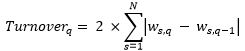
where N is the number of constituents in the index; ws,q–1 and ws,q are the weight (or positions) of stock s in the index at the end of the previous quarter and the beginning of the following quarter, respectively.
In exhibit 2, we report the average annual turnover of the indices. As expected, the turnover of the smart beta indices is much higher than the turnover of their cap-weighted reference benchmark. All the smart beta indices have an annual turnover between 26.90% and 53.67% except for the momentum indices, which have the highest turnover in all the regions and are all above 74%8. Furthermore, we observe that for the emerging markets, turnover of the indices is generally higher than other regions which, added to the fact that the average spread can be expected to be higher as well, may contribute to increased average transaction costs for emerging markets strategies.
Exhibit 2: Average Annual One-Way Turnover
Jun 2002 - Dec 2017
|
Broad CW |
HFI MidCap 4S |
HFI Value 4S |
HFI HighMom 4S |
HFI LowVol 4S |
HFI HighProf 4S |
HFI LowInv 4S |
HFI MBMS6EW 4S |
USA |
3.79% |
42.91% |
34.19% |
78.39% |
30.35% |
30.62% |
40.53% |
36.31% |
GBR |
3.26% |
43.81% |
35.60% |
79.72% |
35.12% |
34.93% |
47.33% |
38.74% |
Dev. EUR ex-UK |
4.57% |
41.26% |
35.00% |
74.92% |
35.15% |
33.31% |
45.03% |
36.65% |
Japan |
3.60% |
36.54% |
33.16% |
77.52% |
33.42% |
26.90% |
43.87% |
34.88% |
Dev. Asia-Pacific ex-Jap |
8.56% |
53.30% |
40.76% |
76.18% |
35.65% |
39.11% |
46.46% |
41.38% |
Emerging |
10.25% |
53.67% |
43.86% |
79.27% |
42.66% |
41.44% |
51.49% |
43.92% |
Global |
4.28% |
44.02% |
36.32% |
78.59% |
34.28% |
33.46% |
44.36% |
37.93% |
This table shows the average turnover of the smart beta indices in our study and their respective cap-weighted reference benchmark. The turnover is calculated as the sum of the absolute deviations of individual weights (or positions) between the end of a quarter and the beginning of the following quarter. For each region, we report the values for each smart beta index and for the reference cap-weighted benchmark in the second column. The period is from December 2002 to December 2017.
In Novy-Marx and Velikov (2016), the authors study the net transaction costs performance of generic academic equity factors which have not been designed to be investable. They show that the net performance of strategies having high turnover, defined as above 50% monthly (600% annually) per month, do not produce significant extra performance relative to the cap-weighted benchmark once the transaction costs are taken into account. Exhibit 2 shows that none of the smart beta indices taken into consideration requires such high levels of turnover.
Transaction Costs and Net Performance
Having shown that the indices in our study have a reasonable level of turnover, we can now investigate if their transaction costs are large enough to significantly deteriorate their performance relative to the cap-weighted benchmark. We start by analysing the performance of all the indices in the seven regions for the same period. We have 15 years of data available, from December 2002 to December 2017.
For each of the smart beta indices and their cap-weighted benchmarks across the seven regions, we show in exhibit 3 the average annualised transaction costs, the gross and net annualised returns relative to the cap-weighted benchmark, and the gross and net Information ratio. We chose to report average transaction costs to give to the reader an idea of how high they may be for investable indices and the net relative returns and Information ratio because they are the measures that allow investors to compare these strategies to an index that requires very little trading such as the cap-weighted benchmark.
Transaction costs are obtained as the difference between the gross return and the net return of the indices. The difference between gross and net returns is only calculated at each rebalancing date. Taking into account weight changes of all stocks at the rebalancing date, the net return of an index is obtained as:
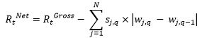
in which RtGross is the gross return, N is the number of stocks, ![]() represent the change in weight from the previous quarter for the stock j, and sj,q is the estimated spread for this stock at the rebalancing date. Our estimates of the spread is the effective spread estimate of Chung and Zhang (2014) based on the closing spread.
represent the change in weight from the previous quarter for the stock j, and sj,q is the estimated spread for this stock at the rebalancing date. Our estimates of the spread is the effective spread estimate of Chung and Zhang (2014) based on the closing spread.
Exhibit 3 shows that the smart beta indices have higher transaction costs than their relative cap-weighted benchmark for all regions. This is due not only to the fact that the turnover is lower in the benchmark but also because the smart beta indices invest higher proportions in relatively smaller stocks, which have higher spreads on average, as we will show in the next section that discusses the determinants of the spreads.
Unsurprisingly, the United States appear to have the most liquid index. The estimates range from 2 basis points for the cap-weighted benchmark to a maximum of 8 basis points for the momentum smart beta index. Looking at the net relative returns, we observe that for all the indices, returns are still high and positive. For instance, the US multi-factor strategy, which has a gross relative return of 2.83% and an Information ratio of 65.73%, is still able to largely outperform the cap-weighted benchmark once transaction costs are taken into account. Indeed, the annualised net relative return is 2.78% and the Information ratio is 64.49%. We observe the strongest deterioration in performance for the momentum index, although it still preserves a positive net relative return of 2.24% and the Information ratio is 40.54%.
The emerging markets have the highest level, on average, of transaction costs. The estimate of the transaction costs ranges from 11 basis points for the cap-weighted benchmark to 25 basis points for the momentum index. Although the transaction costs for this region are quite high, the smart beta indices are still able to outperform the relative benchmark when transaction costs are taken into account. Indeed, all the net relative returns are above 4.2% and in terms of net information ratio, the estimates are all above 55%.
Although the period from 2002 to 2017 includes a major stress on liquidity that happened during the 2007-2008 financial crisis, we extend our analysis further back in time to check that the results discussed above are not dependent on the market conditions of the last 15 years, which is a relatively short period. However, due to data availability issues, we are able to extend our study back in time only for the US market. Furthermore, the closing quotes are only available from 1993. Therefore, we use the Chung and Zhang (2014) methodology for the period after December 1993 and the Corwin and Schultz (2012) methodology from December 1977 to December 1993.
In exhibit 4, we observe that transaction costs over the longer period from 1977 for the US indices amount to 18 basis points per annum for the multi-factor strategy. This long-term assessment can be seen as a conservative estimate of transaction costs, as costs have declined substantially over time. However, even with these long-term estimates of transaction costs, the net relative returns are still high and positive. Across all the measures and indices, net relative returns remain in the range of 2% to 3% and the information ratio in the range of 30% to 50%.
Overall, these results show that transaction cost estimates for the Scientific Beta indices are an order of magnitude smaller than gross outperformance. Thus subtracting estimated costs from returns does not change the conclusions about outperformance of these strategies.
What drives transaction costs?
Hitherto, we have focused on the average transaction cost level of smart beta indices. However, investors are also interested in the determinants of transaction costs. Understanding such determinants is important to judge how costs will differ across time and cross-sectionally. For instance, many studies focus only on the Unites States, which is a highly liquid market. Our results provide information about how easy it is to generalise transaction cost estimates from one region or factor to another. Likewise, time trends in transaction costs are important. If structural changes have led to a reduction in transaction costs, historical estimates could be seen as conservative for example. Furthermore, an investor may be concerned with the possibility of rising transaction costs. During certain time periods, transaction costs may increase, and knowing their sources of commonality helps investors to diversify the risk of such spikes. For example, if transaction costs are mainly driven by regional factors, diversifying across regions may allow the risk of rising transaction costs to be diversified to some extent.
In this section, we analyse the variation of transaction costs from both a time and a cross-sectional perspective. We first show that the average level of transaction costs on the US market decreased after a change in the minimum tick size. Then, we address the question of commonality of transaction costs across regions and factors. We show that there is large commonality across factors and more heterogeneity across regions. Thus, regions are a more important determinant than factors.
Exhibit 3: Average Annualised Transaction Costs
June 2002 - Dec 2017 |
Broad CW |
HFI MidCap 4S |
HFI Value 4S |
HFI HighMom 4S |
HFI LowVol 4S |
HFI HighProf 4S |
HFI LowInv 4S |
HFI MBMS6EW 4S |
USA |
||||||||
Transaction Costs
|
0.02% |
0.06% |
0.05% |
0.08% |
0.04% |
0.04% |
0.05% |
0.05% |
Gross Rel Ret
|
- |
2.99% |
3.49% |
2.32% |
2.80% |
2.64% |
2.56% |
2.83% |
| Net Rel Ret | - | 2.92% |
3.43% |
2.24% |
2.76% |
2.60% |
2.50% |
2.78% |
| Gross IR | - | 63.82% |
79.83% |
42.06% |
46.30% |
57.58% |
53.30% |
65.73% |
| Net IR | - | 62.44% |
78.53% |
40.54% |
45.57% |
56.57% |
52.16% |
64.49% |
UK |
||||||||
Transaction Costs
|
0.06% |
0.13% |
0.13% |
0.19% |
0.11% |
0.12% |
0.15% |
0.12% |
Gross Rel Ret
|
- |
1.50% |
3.37% |
4.01% |
2.78% |
3.71% |
3.63% |
3.22% |
| Net Rel Ret | - | 1.37% |
3.25% |
3.82% |
2.67% |
3.59% |
3.48% |
3.10% |
| Gross IR | - | 17.24% |
48.58% |
51.52% |
35.33% |
48.10% |
49.27% |
47.56% |
| Net IR | - | 15.77% |
46.79% |
49.07% |
33.95% |
46.49% |
47.26% |
45.74% |
Dev. Europe ex-UK |
||||||||
Transaction Costs
|
0.04% |
0.20% |
0.14% |
0.25% |
0.14% |
0.14% |
0.17% |
0.15% |
Gross Rel Ret
|
- |
4.94% |
4.91% |
5.22% |
4.08% |
4.74% |
4.40% |
4.75% |
| Net Rel Ret | - | 4.74% |
4.76% |
4.97% |
3.94% |
4.60% |
4.24% |
4.60% |
| Gross IR | - | 61.34% |
81.76% |
68.83% |
56.38% |
70.83% |
71.46% |
73.77% |
| Net IR | - | 58.97% |
79.43% |
65.67% |
54.54% |
68.89% |
68.84% |
71.55% |
Japan |
||||||||
Transaction Costs
|
0.03% |
0.17% |
0.16% |
0.28% |
0.14% |
0.11% |
0.17% |
0.15% |
Gross Rel Ret
|
- |
4.61% |
5.10% |
3.71% |
4.53% |
4.68% |
4.55% |
4.54% |
| Net Rel Ret | - | 4.45% |
4.94% |
3.43% |
4.40% |
4.57% |
4.38% |
4.39% |
| Gross IR | - | 54.57% |
72.51% |
45.02% |
53.25% |
60.53% |
65.62% |
61.47% |
| Net IR | - | 52.61% |
70.21% |
41.56% |
51.65% |
59.06% |
63.15% |
59.44% |
Dev. Asia-Pacific ex-Japan |
||||||||
Transaction Costs
|
0.06% |
0.45% |
0.30% |
0.52% |
0.27% |
0.29% |
0.33% |
0.31% |
Gross Rel Ret
|
- |
6.34% |
7.16% |
7.87% |
4.53% |
4.99% |
5.57% |
6.09% |
| Net Rel Ret | - | 5.89% |
6.86% |
7.36% |
4.26% |
4.69% |
5.24% |
5.78% |
| Gross IR | - | 78.10% |
101.80% |
108.27% |
56.51% |
74.36% |
79.61% |
92.64% |
| Net IR | - | 72.40% |
97.42% |
101.08% |
53.09% |
69.96% |
74.77% |
87.84% |
Emerging |
||||||||
Transaction Costs
|
0.11% |
0.52% |
0.41% |
0.62% |
0.38% |
0.38% |
0.47% |
0.40% |
Gross Rel Ret
|
- |
5.14% |
4.63% |
4.57% |
4.42% |
4.86% |
4.69% |
4.79% |
| Net Rel Ret | - | 4.62% |
4.21% |
3.94% |
4.04% |
4.48% |
4.22% |
4.39% |
| Gross IR | - | 76.43% |
79.72% |
78.42% |
61.13% |
85.23% |
73.34% |
81.71% |
| Net IR | - | 68.60% |
72.56% |
67.67% |
55.84% |
78.54% |
66.00% |
74.80% |
Global |
||||||||
Transaction Costs
|
0.03%
|
0.16% |
0.13% |
0.21% |
0.12% |
0.12% |
0.14% |
0.13% |
Gross Rel Ret
|
- |
3.72% |
4.11% |
3.59% |
3.41% |
3.62% |
3.47% |
3.68% |
| Net Rel Ret | - | 3.56% |
3.98% |
3.38% |
3.29% |
3.51% |
3.33% |
3.55% |
| Gross IR | - | 97.03% |
128.18% |
83.86% |
69.38% |
95.20% |
91.02% |
100.20% |
| Net IR | - | 92.75% |
124.03% |
78.88% |
67.01% |
92.10% |
87.19% |
96.67% |
This table shows the average annualised transaction cost of the indices, gross relative returns, relative returns net of transaction costs, gross Information ratio and Information ratio net of transaction costs for seven smart beta indices plus a cap-weighted benchmark for seven regions. Transaction costs are computed as the difference between annualised gross and net returns. Net returns are obtained after accounting for transaction costs at each quarterly rebalancing by multiplying the change in weight of each stock between the final weight before rebalancing and the optimal weights after rebalancing by half spread. Gross relative returns and net relative returns are computed subtracting the gross returns of the benchmark. The Information ratios are computed as the ratio of the average relative returns over their standard deviation. The effective spread of each stock in the universe is estimated using the Chung and Zhang (2014) methodology. The period is from December 2002 to December 2017.
Exhibit 4: US Long-Term Results
Dec 1977 - Dec 2017
|
||||||||
Broad CW |
HFI MidCap 4S |
HFI Value 4S |
HFI HighMom 4S |
HFI LowVol 4S |
HFI HighProf 4S |
HFI LowInv 4S |
HFI MBMS6EW 4S |
|
Transaction Costs |
0.01% |
0.22% |
0.18% |
0.35% |
0.17% |
0.16% |
0.20% |
0.18% |
Gross Rel Ret |
- |
2.87% |
2.24% |
3.36% |
2.65% |
2.93% |
2.88% |
2.88% |
Net Rel Ret |
- |
2.65% |
2.06% |
3.02% |
2.49% |
2.78% |
2.68% |
2.70% |
Gross IR |
- |
45.45% |
39.31% |
64.43% |
37.86% |
60.06% |
51.03% |
56.44% |
Net IR |
- |
36.9% |
31.5% |
46.9% |
32.4% |
51.5% |
42.1% |
47.6% |
This table shows the average annualised transaction cost of the indices, gross relative returns, relative returns net of transaction costs, gross Information ratio and Information ratio net of transaction costs for seven smart beta indices plus a cap-weighted benchmark for the United States universe of stocks. Transaction costs are computed as the difference between annualised gross and net returns. Net returns are obtained after accounting for transaction costs at each quarterly rebalancing by multiplying the change in weight of each stock (including stock deletions and additions) between the final weight before rebalancing and the optimal weights after rebalancing by half spread. Gross relative returns and net relative returns are computed subtracting the gross returns of the benchmark. The Information ratios are computed as the ratio of the average relative returns over their standard deviation. The effective spread of each stock in the universe is estimated using the Chung and Zhang (2014) methodology for the period after December 1993 and the Corwin and Schultz (2012) methodology for the previous years. The whole sample period is from December 1977 to December 2017. All the data are obtained from CRSP.
Changes of Transaction Costs Over Time
Between 1997 and 2001, the US stock market went through a change in its market structure. The first change occurred in 1997, when the minimum tick size for a trade went from 1/8th to 1/16th. The second and most significant change occurred in 2001 when the minimum tick size was fixed at 1/100th (i.e. decimalisation). Smaller tick sizes allow for more competitive spreads. Therefore, we would expect a reduction in average spreads.
In exhibit 5, we show the time series of the monthly average effective spread estimator for five size quintiles in the US mid/large cap universe. We can see that there is indeed a general reduction in spread levels if we compare the time periods before and after the most relevant change in tick size that happened in 2001.
It is clear from inspection of the graph that there was a strong reduction in the average effective spread across all stocks in the top 500 universe. Perhaps more importantly, it is apparent that the differences in effective spread reduced tremendously across the size categories. While there was a difference of about 0.5% in the effective spread between the largest capitalisation stocks (highest quintile) and the mid cap stocks (lowest quintile) in the mid-1990s, the difference is barely visible in the graph from 2010. For diversification-based smart beta strategies that will tend to weight stock more evenly across size categories than the cap-weighted index, this means that they have less of a disadvantage over cap-weighted indices in terms of transaction costs.
Given that transaction costs have reduced, and that the reductions can be attributed to structural effects rather than to market conditions, one can argue that historical cost estimates are high compared to cost levels that should be expected currently. Analysing smart beta transaction costs using long time series should thus provide very conservative estimates.
Exhibit 5: Closing Quote Spread Estimates: Top 500 US Stock Universe
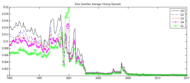
The figure shows the mean monthly spread estimates based on the Closing Quoted Spread Estimator. Reported spreads are mean monthly 2-way spread estimates. Our sample universe consists of the 500 largest ordinary common stocks in the United States in each quarter based on market capitalisation. The daily spread estimate of each stock is estimated based on the chosen estimator. Monthly spreads of each stock are calculated as the average of daily spread estimates of those stocks with at least 12 days of daily spread estimates in a given month. The mean monthly spreads of top decile stocks (largest 10% stocks), bottom decile stocks (smallest 10% stocks) based on market capitalisation and the mean monthly spreads across all stocks in our sample universe are reported for each type of estimator. The period is from December 1993 to December 2017. Data Source: CRSP.
Factors vs. Regions
Understanding the drivers of transaction costs is important for investors in order to judge the relevance of results for a given strategy and in order to assess possibilities for diversifying the risk of variations in transaction costs. Other papers have studied what the sources of commonalities driving the transaction costs are. Chordia et al. (2000) showed empirically that there are common movements in the liquidity of the assets on the US market. Quoted spreads of individual assets co-move with market and industry-wide liquidity measures. Hasbrouck and Seppi (2001) use a principal component analysis to show that there are common factors explaining the cross-section of the order flows of individual assets. Brunnermeier and Pedersen (2009)9 link the commonality in transaction costs across assets to funding liquidity conditions. Such conditions are likely to differ across regions, suggesting a strong role for regions as drivers of transaction costs.
We investigate this intuition by analysing the correlation between transaction costs and the weighted average spread of the Scientific Beta indices.
Exhibit 6 shows the percentage of the variance explained by principal components obtained using the seven global indices (factors) and the MBMS6EW index in the seven regions considered in this analysis. The figure shows that the principal components extracted from regions have a slower convergence to 100% of explained variance than principal components extracted from factors. Thus, regions show less commonality in costs than factors.
Exhibit 6: Principal Component Analysis of Transaction Costs
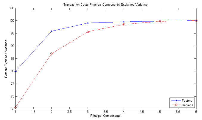
This figure shows the explained variance of the principal components of the transaction costs of Scientific Beta indices. We obtain the ‘Factors’ principal components using the transaction costs of 8 Global indices on different factors and the ‘Regions’ principal components using the transactions costs of the MBMS6EW Index for 7 different regions. For the transaction costs, we use the closing spread as an estimate of the effective spread. Analytics are calculated over the period 31 December 2002 to 31 December 2017.
For investors, these findings imply that they need to think carefully about transaction costs when applying a smart beta strategy to a different region. Since regions are a main driver of transaction costs, results and experiences obtained with a strategy in one region may not carry over to another region. On the other hand, factors display stronger commonality, suggesting that there is less impact of a factor choice on the behaviour of transaction costs. Moreover, for investors who are concerned about possible adverse variations in transaction costs over time, diversifying across regions may provide better potential to smooth transaction costs over time.
Conclusions
Our results show that the outperformance of smart beta strategies relative to the cap-weighted benchmark is robust to accounting for transaction costs. These results hold for strategies that are invested in the most liquid universes of stocks and that adopt turnover controls and liquidity rules to limit trading. We have shown that relative returns and Information ratio are still high and positive when assessing net-of-cost results. This finding holds across several regions including emerging markets. We also find positive net-of-cost performance in the US universe when considering a longer time period with higher cost levels than over the recent period.
We have also shown that the average cost of trading, measured in terms of effective spread, has decreased in the last decade, as the market structure has improved, in particular through the reduction in the minimum tick size for trading. Therefore, historical cost estimates carry an upward bias compared to costs faced today by investors. Analysing smart beta strategies using long time series provides a conservative estimate of transaction costs.
Finally, we have shown that the correlation in transaction costs is stronger across factors than across regions. This result is consistent with the theoretical literature and implies that investors may decrease exposure to time variation in transaction costs of smart beta strategies by being well diversified across regions.
All our results have been obtained using transparent and easily replicable methodologies for the measurement of transaction costs. We hope that our effort will allow for a wider use of replicable transaction cost measures of smart beta strategies. When considering different smart beta strategies, investors should be able to get information not only on factor exposures and past performance. Given that any smart beta strategy requires rebalancing of stock weights, investors should also be able to get replicable insights into transaction costs of candidate strategies.
Footnotes:
1A detailed description of these critiques may be found in Amenc et al. (2016).
2For instance Frazzini et al. (2015).
3An example is Novy-Marx and Velikov (2016), in which the authors analyse long/short decile strategies. Although, they also show that using controls that reduce implementation issues improves the net performance of factor strategies.
4We also note that, other than commissions, our analysis will not include cost categories such as financial transaction taxes, exchange taxes, or a stamp duty which may exist in certain markets. Moreover, taxes that may be applicable at the level of the investor (e.g. taxes on realised capital gains) that may also differ depending on rebalancing schedules and implementation approach are not considered. In fact, such taxes may vary depending on the status of the investor which would make it challenging to include them in the analysis.
5They align well with the spread measures obtained from high frequency data. Holden (2009) provides a rather comprehensive analysis of these measures.
6Scientific Beta is a smart beta index provider set up by EDHEC-Risk Institute as part of its policy of transferring know-how to the industry. Scientific Beta is an initiative which aims to favour the adoption of the latest advances in smart beta design and implementation by the investment industry.
7The reason to report the one-way turnover instead of the two-way is because we estimate the full spread and the way to compute the cost of a round-trip transaction is to multiply the full spread for the one-way turnover.
8Momentum indices have higher turnover because it loads on the momentum score that is recomputed more frequently, semi-annually, whereas all the other factor scores are recomputed on an annual basis.
9They approach the question from a theoretical point of view and develop a model to explain commonality in transaction costs. They start from the assumption that trading requires capital to be posted because of margin requirements. The funding of market dealers affects their ability to trade, hence to provide liquidity on the market. Therefore, negative shocks to the funding liquidity of the dealers of a certain market also deteriorates the market liquidity of the stocks on that specific market. If the main source of cross-sectional correlation in transaction costs is the funding liquidity of the dealers, and if the funding liquidity of dealers in different regions is not perfectly correlated, strategies investing in stocks in the same regions should have a higher correlation in transaction costs than strategies investing in different regions.